Interpreting single-cell RNA-seq data: from count matrix to biological hypothesis

Key analysis considerations that help researchers move from raw single-cell RNA-seq counts to cell type assignments, differential expression results, and pathway-level hypotheses.

Single-cell RNA sequencing can reveal biology that gets lost with bulk approaches due to averaging (as we covered extensively in this Single-cell Analysis MiniBootcamp). It can uncover rare cell populations, cell-state changes, and condition-specific gene expression patterns. But the path from a cell-by-gene count matrix to a clear biological interpretation is rarely straightforward.

One filtering decision can change clustering. One clustering parameter can change cell type assignments. One cell type assignment can change which genes appear significant. As decisions stack up across analysis, it can become difficult to explain how the final results were reached.

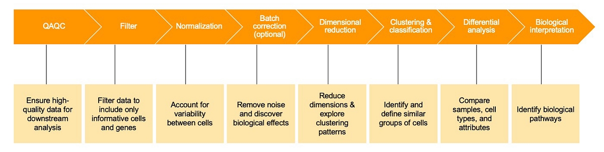
An interpretation-focused guide helps reduce that complexity by giving each decision a clear purpose: 

• Remove low-quality cells
• Focus on informative genes
• Normalize technical differences
• Reveal structure
• Assign cell identities
• Test focused comparisons
• Interpret results in biological context 

Clear analysis context helps make that process easier to review and explain. If a pathway appears important at the end, researchers need to know which cells were filtered, how clusters were defined, which markers supported classification, and which model generated the differential expression results. A connected environment helps keep decisions, visualizations, and results easier to follow as the analysis progresses.

Use this guide as an interpretation framework for understanding the analysis decisions that connect single-cell RNA-seq counts to cell types, differential expression results, and pathway-level hypotheses. 

A working example: aging-associated changes in dorsal root ganglia

To illustrate these analysis considerations, this blog uses dorsal root ganglia samples from three-month-old and 21-month-old mice generated with the Illumina Single Cell 3’ RNA Prep, T20 kit. The example is demonstrated in Illumina Connected Multiomics (start a free trial), a software environment that enables researchers to review single-cell RNA-seq analysis steps, outputs, and visualizations in one place. The analysis asks three questions: do cell type frequencies change with age, which genes differ between younger and older samples, and which pathways help explain those changes? The same approach can be adapted to other single-cell RNA-seq studies.

Step 1: Review cell quality before making comparisons

Start by asking whether the cells are suitable for downstream analysis. Common QC metrics include total counts, detected genes, percent mitochondrial counts, and percent ribosomal counts. Together, these metrics help flag low-quality cells, damaged cells, dead or dying cells, potential doublets, and other technical artifacts.

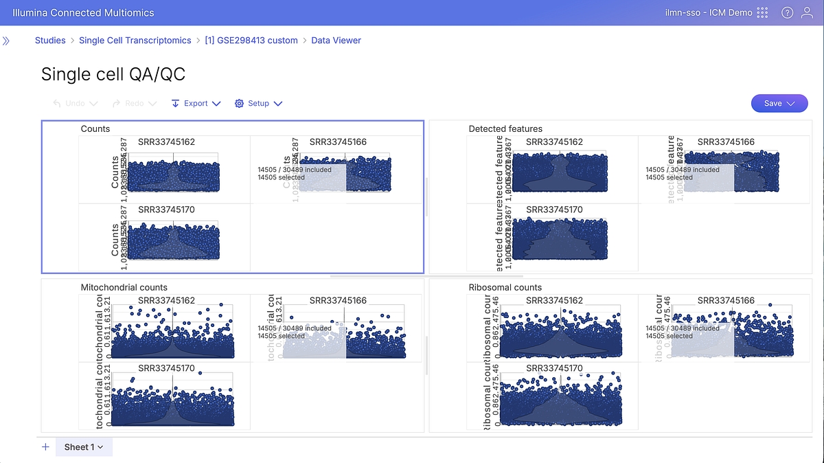
Thresholds should be chosen in context. Low counts and few detected genes may indicate poor-quality cells. Very high counts and many detected genes may indicate doublets. A high mitochondrial percentage can suggest damage, but it may also be expected in some tissues or cell types. In the dorsal root ganglia aging example, the goal is to remove cells likely to distort clustering or differential analysis without filtering out biology that may matter.

Why it matters: QC decisions shape every downstream result, so filtering should account for both data quality and biological context.

Step 2: Filter features to reduce noise without losing signal

Next, evaluate the genes or features that will carry forward. Not every measured gene adds useful biological signal. Some genes may contribute little variation, while others may add noise or computational burden without improving interpretation.

Feature filtering helps focus the analysis on informative genes. Highly variable gene selection is often useful because it retains genes that help distinguish cells and support downstream structure detection. The balance is important: overly strict thresholds can remove markers for rare or biologically important populations before those populations are recognized.

Why it matters: Feature filtering reduces noise while preserving the genes needed for clustering, classification, comparison, and interpretation.

Step 3: Normalize expression values before comparing cells

Normalization helps account for technical differences between cells, especially differences in sequencing depth. Instead of comparing raw counts directly, normalization adjusts expression values so cells can be compared more fairly.

A typical approach adjusts counts for sequencing depth, applies a scale factor, adds an offset to manage zero values, and uses a log transformation to compress expression values. Other methods, such as SCTransform or scran deconvolution, may be appropriate depending on the data set and analysis strategy. Normalizing after filtering helps prevent low-quality cells or low-information features from shaping the normalized data structure.

Why it matters: Normalization helps reduce technical differences that can obscure biological variation.

Step 4: Check for batch effects before correcting them

Batch correction can help when technical artifacts make samples appear different for reasons unrelated to the biological question. Samples processed on different days, prepared by different operators, or generated across studies may show structure driven by technical variation.

Before correcting, look for evidence that correction is needed. PCA and other exploratory views can show whether samples separate by technical factors. If cells from different samples occupy separate regions when they should overlap, technical artifacts may be influencing the analysis. But batch correction is not risk-free: overcorrection can weaken or remove real biology.

Why it matters: Batch correction should reduce unwanted technical variation without removing the biological structure needed to answer the research question.

Step 5: Use dimension reduction to inspect structure

Single-cell data is too high dimensional to interpret directly. Dimension reduction projects many genes across many cells into fewer dimensions so researchers can inspect structure, identify outliers, evaluate sample relationships, and prepare for clustering.

PCA is often used first to capture major sources of variation, and a scree plot can help decide how many principal components to carry forward. UMAP and t-SNE then provide complementary views of finer-scale structure. In the dorsal root ganglia example, these views help assess whether cells organize by sample group, cell population, or possible technical effects.

Why it matters: Dimension reduction is a checkpoint that helps confirm the analysis is moving in a sensible direction.

Step 6: Cluster cells, then validate what the clusters mean

Clustering groups cells with similar expression profiles, but the output depends on analysis choices such as resolution, number of principal components, and number of nearest neighbors. Because those choices can change the number and composition of clusters, clustering should be treated as iterative.

Clusters are useful, but they are not automatically cell types. Marker genes, computed biomarkers, tissue biology, and automated classification tools can all support cell identity assignments. In Illumina Connected Multiomics, tools such as ScType and Garnett can be used alongside manual marker review.

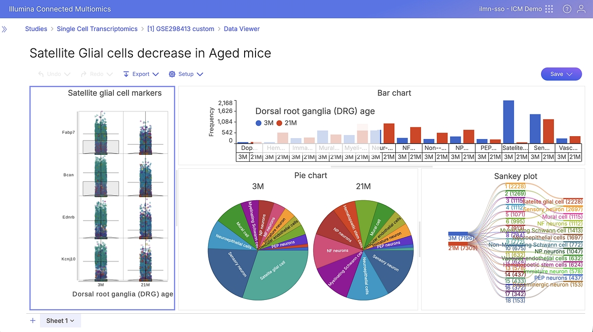
In the dorsal root ganglia example, classification enables comparison of cell type frequencies between three-month-old and 21-month-old mice. A decrease in satellite glial cells in the older group becomes easier to evaluate when cluster maps, marker expression, frequency plots, and labels are reviewed together.

Why it matters: Clustering reveals structure; classification gives that structure biological meaning.

Step 7: Test focused comparisons

Once cell populations are defined, differential analysis lets researchers ask focused biological questions. In the dorsal root ganglia example, one comparison is gene expression in satellite glial cells from 21-month-old mice versus three-month-old mice.

Model choice should match the comparison. For single-cell data, a hurdle model can be useful because it supports multivariate comparisons and accounts for zero-heavy expression values. Other models, such as Wilcoxon, may fit different use cases. After the comparison runs, researchers can filter results by statistical significance, corrected p-value, fold change, or criteria aligned to the study design.

Why it matters: Tying comparisons to defined cell populations keeps gene changes in the right biological context.

Step 8: Add pathway-level interpretation

After differential analysis, pathway interpretation helps move from a gene list to broader biological context. KEGG pathway enrichment and Correlation Engine pathway analysis can identify pathways or gene sets overrepresented among differentially expressed genes.

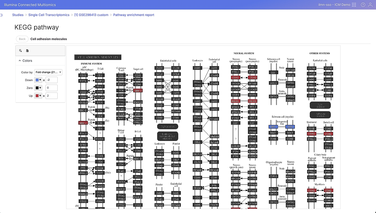
In the dorsal root ganglia example, enriched pathways such as cell adhesion molecules can support hypothesis generation about cell function, microenvironment regulation, or injury response during aging. These pathway-level views help researchers move beyond individual genes and focus on biological patterns that can guide follow-up questions.

Why it matters: Pathway interpretation connects gene-level results to biological hypotheses that can guide follow-up studies.

Bringing the analysis decisions together

Single-cell RNA-seq analysis is easier to interpret when each step connects to the next. 

• QC and filtering shape the data that moves forward, helping focus the analysis on suitable cells and informative genes.
• Normalization and optional batch correction prepare the data for structure discovery, helping reduce technical effects before dimensional reduction.
• Dimensional reduction, clustering, and classification turn structured data into defined cell populations, making it possible to interpret cell types and states.
• Differential analysis uses those defined populations to compare samples, cell types, or other attributes, helping identify gene-level changes tied to the study question.
• Biological interpretation builds on those gene-level results, connecting differential expression patterns to pathways and broader study context.

For researchers who want to keep those analysis decisions easier to review, Illumina Connected Multiomics provides a connected environment for single-cell RNA-seq analysis. The software brings analysis tasks, outputs, visualizations, and results together so teams can follow how data moves from cell-level counts to cell populations, differential genes, and pathway-level hypotheses.

In the dorsal root ganglia example, that connected context makes it easier to review the choices behind the final interpretation, including which cells were retained, how clusters were classified, which comparison was tested, and which pathways were identified for follow-up. It also helps researchers revisit earlier decisions when a downstream result raises new questions.

Explore connected single-cell analysis in Illumina Connected Multiomics

Illumina Connected Multiomics supports single-cell RNA-seq analysis from quality control and normalization through dimensional reduction, clustering, classification, differential analysis, and biological interpretation. By keeping key steps and results in one environment, researchers can more easily review analysis decisions, share context, and connect gene-level findings to pathway-level hypotheses.

To continue learning, watch the Single-cell Analysis MiniBootcamp for a deeper dive into the analysis steps covered in this guide. If you are ready to explore your own data, start an instant free 30-day trial of Illumina Connected Multiomics and apply the same connected approach to your own study.

---

For Research Use Only. Not for use in diagnostic procedures.

M-GL-04757